Analyzing the Netflix dataset

Introduction

After beating the giant Blockbuster in the 2000s, Netflix established itself as the top provider of movies; firstly by shipping DVDs and then by becoming one of the first adopters of streaming content online that paved the way into its success today.

Being part of our digital life, we will be analyzing its dataset provided by Datacamp.

Data Description

netflix_data.csv

Column	Description
`show_id`	The ID of the show
`type`	Type of show
`title`	Title of the show
`director`	Director of the show
`cast`	Cast of the show
`country`	Country of origin
`date_added`	Date added to Netflix
`release_year`	Year of Netflix release
`duration`	Duration of the show in minutes
`description`	Description of the show
`genre`	Show genre

Used Libraries

import pandas as pd
import numpy as np
import plotly.express as px
import seaborn as sns
import matplotlib.pyplot as plt
import matplotlib.font_manager as fm
from pathlib import Path

Data Cleaning

To ensure data quality, we have to inspect the dataset first and clean its records in order to obtain viable data.

data = pd.read_csv('netflix_data.csv')
data.info()

<class 'pandas.core.frame.DataFrame'>
RangeIndex: 4812 entries, 0 to 4811
Data columns (total 11 columns):
 #   Column        Non-Null Count  Dtype 
---  ------        --------------  ----- 
 0   show_id       4812 non-null   object
 1   type          4812 non-null   object
 2   title         4812 non-null   object
 3   director      4812 non-null   object
 4   cast          4812 non-null   object
 5   country       4812 non-null   object
 6   date_added    4812 non-null   object
 7   release_year  4812 non-null   int64 
 8   duration      4812 non-null   int64 
 9   description   4812 non-null   object
 10  genre         4812 non-null   object
dtypes: int64(2), object(9)
memory usage: 413.7+ KB

df = data.copy()

Upon trying to convert the column date_added, we notice that there is an error in the 161st row where the date has a space at the beginning of the string.

pd.to_datetime(df['date_added']) time data " August 4, 2017" doesn't match format "%B %d, %Y", at position 161.

df[df['date_added'].str.startswith(' ')][['title', 'date_added']]

                title         date_added
203   Abnormal Summit     August 4, 2017
1339     Father Brown     March 31, 2018
2477             Mars   November 1, 2019
3292      Royal Pains       May 18, 2017

#4 records that can cause problems as they start with a space
df['date_added'] = df['date_added'].str.lstrip()
#Verifying
df[df['date_added'].str.startswith(' ')]

Empty DataFrame
Columns: [show_id, type, title, director, cast, country, date_added, release_year, duration, description, genre]
Index: []

#It now works fine
pd.to_datetime(df['date_added'])

0      2016-12-23
1      2018-12-20
2      2017-11-16
3      2020-01-01
4      2017-07-01
          ...    
4807   2019-11-01
4808   2018-07-01
4809   2020-01-11
4810   2020-10-19
4811   2019-03-02
Name: date_added, Length: 4812, dtype: datetime64[ns]

After cleaning the column and turning to the duration one, we spot a bizarre duration of potentially 1 minute for some shows which could cause problems.

After inspecting the data, it seems that we have two types of shows; Movies and TV Shows where the latter has the same odd duration records due to shows typically being measured with the number of seasons/episodes.

df[['title', 'duration']].sort_values('duration').head()

                                 title  duration
1935                       Jack Taylor         1
2411  Maggie & Bianca: Fashion Friends         1
1879                 Inhuman Resources         1
2956                   Paava Kadhaigal         1
2942       Ouran High School Host Club         1

#it appears that TV shows have incorrect durations which is logical due to them having many episodes
df[df['type'] == 'TV Show']['duration'].describe()

count    135.000000
mean       1.940741
std        2.118726
min        1.000000
25%        1.000000
50%        1.000000
75%        2.000000
max       15.000000
Name: duration, dtype: float64

#To insure that all the data for tv shows is incorrect we will check the TV show with the longest duration
df.iloc[df[df['type'] == 'TV Show']['duration'].idxmax()]

show_id                                                     s5913
type                                                      TV Show
title                                                Supernatural
director                                            Phil Sgriccia
cast            Jared Padalecki, Jensen Ackles, Mark Sheppard,...
country                                             United States
date_added                                           June 5, 2020
release_year                                                 2019
duration                                                       15
description     Siblings Dean and Sam crisscross the country, ...
genre                                                     Classic
Name: 3678, dtype: object

In order to make sure that our assumption is correct, we will explore communicating with an LLM model in two ways to verify the duration of the TV show with the longest duration: Supernatural.

Code for communicating with Qwen2.5 using HuggingFace’s API to get verify the duartion.

from huggingface_hub import InferenceClient

file = open('api.txt', 'r')
api = file.read()
file.close()

client = InferenceClient(api_key=api)

messages = [
    {
        "role": "user",
        "content": "What is the duration of the TV Show Supernatural?"
    }
]

stream = client.chat.completions.create(
  model="Qwen/Qwen2.5-Coder-32B-Instruct", 
    messages=messages, 
    max_tokens=500,
    stream=True
)

for chunk in stream:
    print(chunk.choices[0].delta.content, end="")

The TV show “Supernatural” originally aired from September 13, 2005, to May 22, 2022, consisting of 15 seasons, with a total of 327 episodes. Each episode is typically 46 minutes in length, including commercials in the United States.

Alternativly, we can use the R package {ollamar} to communicate with a locally installed LLM model in order to get answers.

set.seed(21)
generate("llama3.2", 
         "What is the duration of the TV Show Supernatural? Answer it shortly and concisely.", 
         output = "text")

[1] “The TV show Supernatural ran for 15 seasons from September 2005 to November 2019, with a total of 327 episodes.”

According to the answers provided by the two models, the duration column for TV shows is mainly for the number of seasons available on Netflix which causes us to separate movies and TV shows into two different dataframes.

tv_shows = df[df['type'] == 'TV Show']
movies = df[df['type'] != 'TV Show']

Data Extraction

For this part of the report, we will be transforming data which we will use to create visualizations and highlight interesting insights from the dataset.

Extracting the Top 10 Most Productive Countries

top_10_countries = df.groupby('country').size().sort_values(ascending = False).head(10)

Extracting the Top 10 Directors Info

An interesting analysis would be to analyze the most productive directors from their favorite actor to their most produced genre.

df_expanded = df.assign(actors=df['cast'].str.split(', ')).explode('cast')

top_10_directors = df_expanded.groupby('director').size().sort_values(ascending=False).head(10)

#A function to get the most produced genre for each director
def top_genre(x):
    return x.mode().iloc[0] if not x.empty else None

#Function to get most casted actor by each director
def most_common_actor(actors_column):
    all_actors = [actor for actors_list in actors_column for actor in actors_list]
    return pd.Series(all_actors).mode().iloc[0] if all_actors else None

director_analysis = pd.DataFrame({
    'num_shows': top_10_directors,
    'most_produced_genre': df_expanded.groupby('director')['genre'].apply(top_genre),
    'mean_duration': df_expanded.groupby('director')['duration'].mean().round(2),
    'favorite_actor': df_expanded.groupby('director')['actors'].apply(most_common_actor)
}).loc[top_10_directors.index]

#Reset index to make the director's a column
director_analysis = director_analysis.reset_index()

#Rename columns for clarity
director_analysis = director_analysis.rename(columns={
    'director': 'Director',
    'num_shows': 'Number of Shows',
    'most_produced_genre': 'Most Produced Genre',
    'mean_duration': 'Average Duration',
    'favorite_actor': 'Most Featured Actor'
})

Extracting Holiday-themed Movies

holiday_movies = df[df['title'].str.contains('Christmas|Holiday|Santa|Xmas|Easter|Thanksgiving|New Year', case=False, na=False)].reset_index()

Adding a sentiment column would be useful for those who want ‘happy vibes’ movies instead of an action packed one.

R code to communicate with a locally installed Llama 3.2 to extract sentiments using the {mall} package.

llm_use("ollama", "llama3.2")

── mall session object

Backend: ollama
LLM session: model:llama3.2
R session: cache_folder:/tmp/Rtmp7UNNqV/_mall_cache12f8922c024e9

R code to communicate with a locally installed Llama 3.2 to extract sentiments using the {mall} package.

holiday_movies_t <- reticulate::py$holiday_movies |>
  select(title, genre, release_year, duration, description) |>
  llm_sentiment(col = description, 
                pred_name = 'sentiment', )

R code for creating the following table.

library(reactable)
library(dplyr)
library(htmltools)

get_duration_color <- function(duration) {
  color_pal <- function(x) rgb(colorRamp(c("#9fc7df", "#416ea4"))(x), maxColorValue = 255)
  normalized <- (duration - min(duration)) / (max(duration) - min(duration))
  color_pal(normalized)
}

get_sentiment_color <- function(sentiment) {
  color_pal <- function(x) rgb(colorRamp(c("#ff6b6b", "#4ecdc4", "#f5f5dc"))(x), maxColorValue = 255)
  
  # Create a numeric mapping for sentiments
  sentiment_mapping <- factor(sentiment, levels = c("negative", "positive", "neutral"))
  normalized <- ifelse(is.na(sentiment_mapping), 0.5, 
                       (as.numeric(sentiment_mapping) - 1) / (nlevels(sentiment_mapping) - 1))  
  color_pal(normalized)
}

holiday_movies_t <- holiday_movies_t %>%
  select(title, genre, release_year, duration, sentiment) %>% 
  mutate(duration_color = get_duration_color(duration),
         sentiment_color = get_sentiment_color(sentiment))

holiday_movies_table <- reactable(
  holiday_movies_t,
  defaultColDef = colDef(
   vAlign = "center", 
   headerClass = "header",
   style = list(fontFamily = "Karla, sans-serif")
  ),
  columns = list(
    title = colDef(
      name = "Movie Title",
      minWidth = 250
    ),
    genre = colDef(
      name = "Genre",
      minWidth = 100
    ),
    release_year = colDef(
      name = "Year",
      defaultSortOrder = "desc",
      width = 80
    ),
    duration = colDef(
      name = "Duration",
      defaultSortOrder = "desc",
      cell = function(value, index) {
        color <- holiday_movies_t$duration_color[index]
        div(
          style = sprintf(
            "background-color: %s; border-radius: 4px; padding: 4px; color: black;",  
            color
          ),
          value
        )
      },
      width = 120
    ),
    sentiment = colDef(
      name = "Sentiment",
      cell = function(value, index) {
        color <- holiday_movies_t$sentiment_color[index]
        div(
          style = sprintf(
            "background-color: %s; border-radius: 4px; padding: 4px; color: black;",  
            color
          ),
          value
        )
      },
      width = 140
    ),
    duration_color = colDef(show = FALSE),
    sentiment_color = colDef(show = FALSE)
  ),
  highlight = TRUE,
  language = reactableLang(
    noData = "No Holiday movies found",
    pageInfo = "{rowStart}\u2013{rowEnd} of {rows} Holiday movies"
  ),
  theme = reactableTheme(
    searchInputStyle = list(
              backgroundColor = "#f7e9de"
            ),
    backgroundColor = "transparent",
    color = "#333333",
    highlightColor = "rgba(0, 0, 0, 0.05)",
    borderColor = "rgba(0, 0, 0, 0.1)",
    headerStyle = list(
      backgroundColor = "transparent", 
      borderColor = "rgba(0, 0, 0, 0.1)",
      borderBottomWidth = "2px",
      fontWeight = "600"
    )
  ),
  class = "holiday-movies-tbl",
  searchable = TRUE,
  striped = TRUE,
  defaultPageSize = 10,
  style = list(fontFamily = "Karla, sans-serif")
)

holiday_movies_table

Data Visualization

The scene on Netflix is expectedly dominated by Americans with a surprising 2nd place for India that is logical after remembering the rise of Bollywood these recent years.

Code

movies_per_country = df['country'].value_counts()

fig = px.choropleth(locations=movies_per_country.index, 
                    locationmode='country names',
                    color=movies_per_country.values,
                    title='Netflix Production Distribution Across Countries',
                    color_continuous_scale = 'Blues')

fig.update_layout(
  coloraxis_showscale=False,
  font_family = 'Karla',
    geo=dict(
        showframe=False,
        showcoastlines=True,
        projection_type='equirectangular',
        landcolor='lightgray',
        showcountries=True,
        countrycolor='white',
        oceancolor='aliceblue'
    )
)

Most movies on Netflix are newish ranging from 2016 to 2018 which were their most active years, but they since got more selective to favor quality shows.

Code

shows_per_year = df.groupby('release_year').size().reset_index(name='count')

fig = px.bar(shows_per_year, x='release_year', y='count', 
             title='Distribution of Netflix Shows/Movies release years',
             labels={'release_year': 'Release Year', 'count': 'Number of Shows'})
             
fig.update_layout(font_family = 'Karla')

Movies on Netflix are mostly Dramas and Comedies with both genres taking up 52.3% of the dataset, with Action coming up third with 15.4% and surprisingly the Children genre being fourth with 421 shows!

The Top 3 are expected from a platform like Netflix which was always known for its drama-packed and intriguing series/movies.

Code

genre_counts = df['genre'].value_counts()[df['genre'].value_counts() > 50]

fig = px.pie(values=genre_counts.values, 
             names=genre_counts.index, 
             title='Distribution of Genres')

fig.update_layout(font_family = 'Karla')

Starting with a rather balanced catalog, Netflix went on to focus on Drama and Comedy which paved their way into success and more attraction.

Code

font_path = Path('KarlaRegular.ttf')

karla_font = fm.FontProperties(fname=font_path)
fm.fontManager.addfont(font_path)

plt.rcParams['font.family'] = karla_font.get_name()
plt.rcParams['axes.spines.right'] = False
plt.rcParams['axes.spines.top'] = False

genre_yearly = df.groupby(['release_year', 'genre']).size().unstack(fill_value=0)

top_genres = genre_yearly.sum().nlargest(5).index

plt.figure(figsize=(12,6))
for genre in top_genres:
    plt.plot(genre_yearly.index, genre_yearly[genre], label=genre)

fig = plt.gcf()
fig.patch.set_alpha(0)
ax = plt.gca()
ax.set_facecolor('#CCC1B7')
plt.title('Top 5 Genres Over the Years',
  fontsize=20,
  fontweight='bold',
  color='#333333')
plt.xlabel('Year')
plt.ylabel('Number of Shows')
plt.xlim(1940, 2021);
ax.locator_params(axis='x', nbins=16)
plt.legend()
plt.show()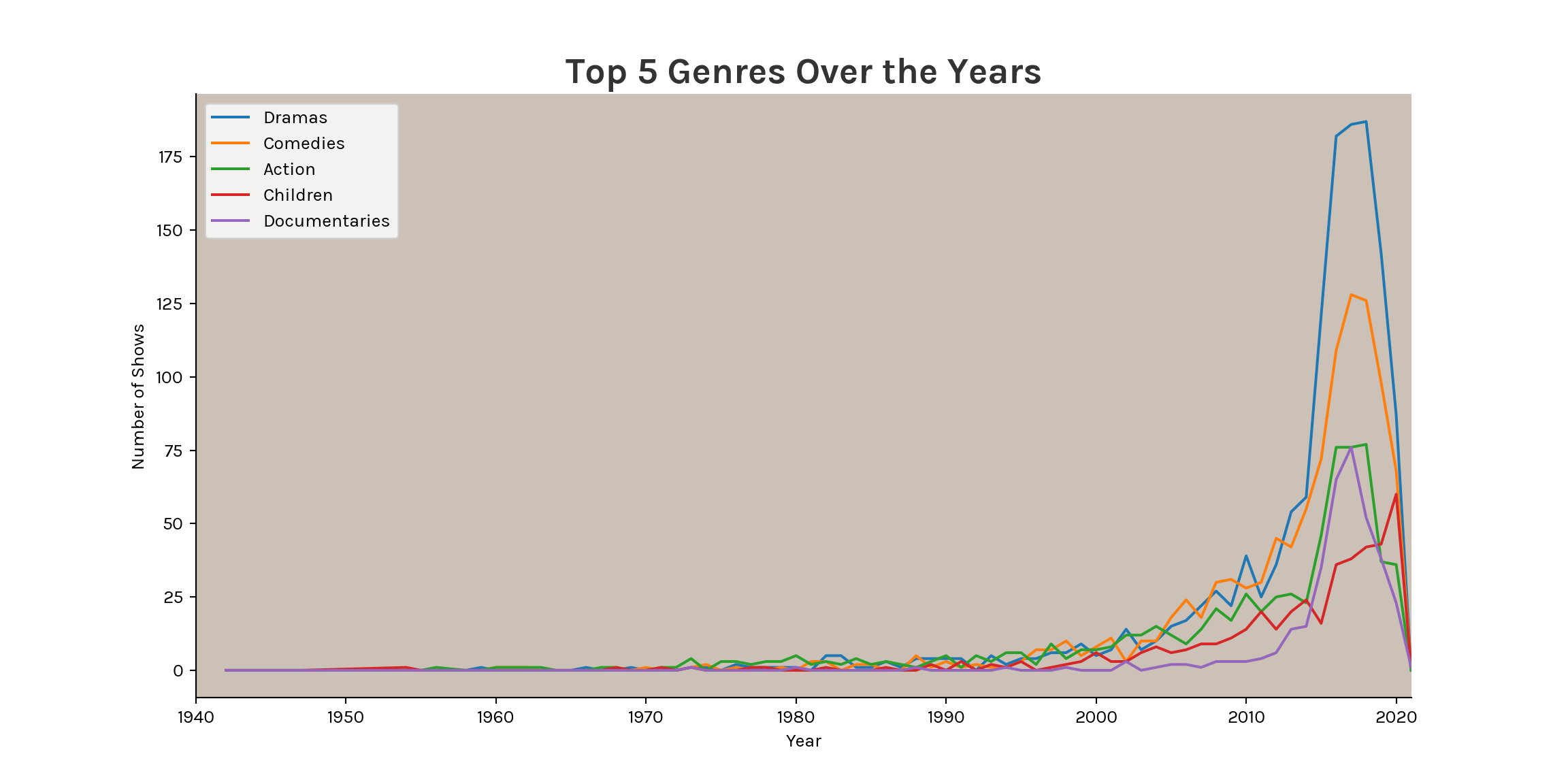

Interestingly, 5 out of the Top 10 directors primarily produce stand-ups! Which is kind of expected because stand-ups don’t require much effort compared to movies but surprising when we check the previous plot that has stand-ups as the 6th most produced genre with 283 shows.

Code

font_path = Path('KarlaRegular.ttf')

karla_font = fm.FontProperties(fname=font_path)
fm.fontManager.addfont(font_path)

plt.rcParams['font.family'] = karla_font.get_name()
plt.rcParams['axes.spines.right'] = False
plt.rcParams['axes.spines.top'] = False

fig, ax = plt.subplots(figsize=(12, 8))
ax.set_facecolor('#CCC1B7')
fig.patch.set_alpha(0)

# def apply_dark_mode(ax, fig):
#     for text in ax.texts:
#         text.set_color('white')
#         
#     ax.tick_params(axis='x', colors='white')
#     ax.tick_params(axis='y', colors='white')
#     
#     for label in ax.get_yticklabels():
#         label.set_color('white')
#     
#     for label in ax.get_xticklabels():
#         label.set_color('white')
#     
#     for figtext in fig.texts:
#         figtext.set_color('white')
#         
# if dark_mode:
#     apply_dark_mode(ax, fig)

top_directors = director_analysis['Director'].values
df_filtered = df[df['director'].isin(top_directors)]
genre_counts = df_filtered.groupby(['director', 'genre']).size().unstack(fill_value=0)
genre_proportions = genre_counts.div(genre_counts.sum(axis=1), axis=0)
genre_proportions = genre_proportions.reindex(top_directors[::-1])

custom_colors = {
    'Action': '#a10000',       
    'Children': '#093803',     
    'Classic Movies': '#4b4b4b', 
    'Comedies': '#298605',
    'Documentaries': '#633103', 
    'Dramas': '#904fb6',
    'International Movies': '#00a2ff',
    'Stand-Up': '#1f5383'
}

director_counts = df['director'].value_counts().head(10)
left = np.zeros(len(top_directors))
directors = top_directors[::-1] 
counts = director_counts.values[::-1] 

for genre in genre_proportions.columns:
    width = counts * genre_proportions[genre].values
    bars = ax.barh(range(len(directors)), width, left=left, 
                   color=custom_colors[genre], alpha=0.9, label=genre)
    
    for i, bar in enumerate(bars):
        percentage = genre_proportions[genre].values[i] * 100
        if percentage >= 5:
            center = left[i] + width[i]/2
            ax.text(center, i, 
                   f'{genre}\n{percentage:.1f}%',
                   ha='center',
                   va='center',
                   fontsize=8,
                   color='white')
    
    left += width

ax.text(0, 1.1, 'Top 10 Most Productive Directors',
        transform=ax.transAxes,
        fontsize=20,
        fontweight='bold',
        color='#333333')

ax.text(0, 1.05, 'Number of titles directed by each director, with genre distribution',
        transform=ax.transAxes,
        fontsize=14,
        color='#333333',
        alpha=0.8)

ax.tick_params(axis='both', colors='#333333')
ax.tick_params(axis='y', length=0)

plt.xlim(0, 18);
ax.locator_params(axis='x', nbins=9)
ax.grid(True, axis='x', linestyle='--', alpha=0.2, color='#666666')
ax.grid(False, axis='y')

plt.ylabel('')
ax.set_yticks(range(len(directors)))
ax.set_yticklabels(directors)

for i, v in enumerate(counts):
    ax.text(v + 0.2, i,
            str(int(v)),
            va='center',
            fontsize=10,
            color='#333333')

plt.legend(bbox_to_anchor=(1.05, 1), loc='upper left', fontsize=8)

plt.figtext(0.85, 0.02, 'Source: DataCamp Datasets',
            fontsize=9,
            color='#333333',
            alpha=0.7)

plt.tight_layout()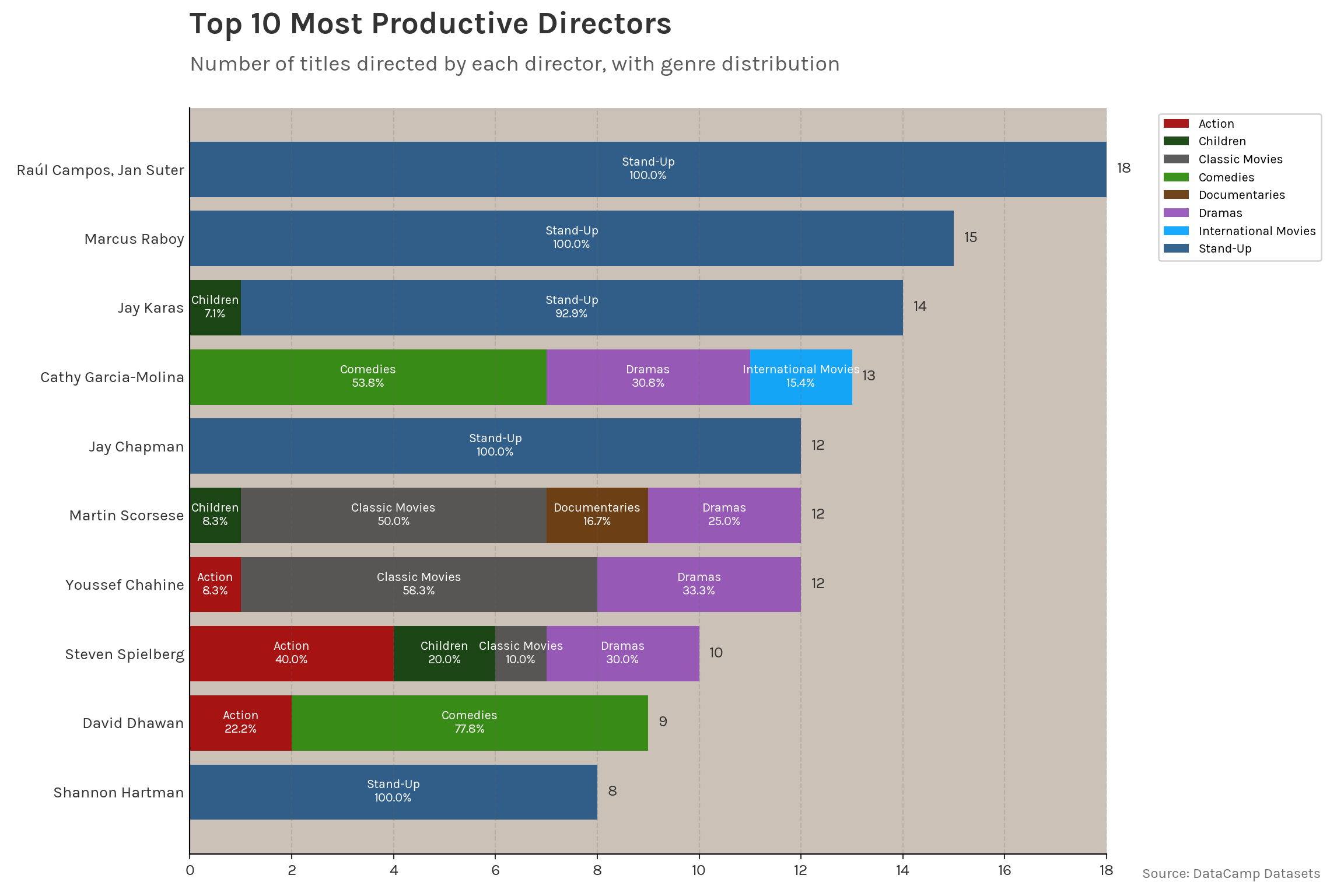

Further analysis highlights the difference of genres mostly seen in the average duration and the most featured actors where you see renowned names like Harrison Ford compared to the near unknown names! (except for Bill Burr of course.)

R code to display the following table.

library(gt)
library(gtExtras)

add_text_img <- function (text, url, height = 30, left = FALSE) {
  text_div <- glue::glue("<div style='display:inline;vertical-align: top;'>{text}</div>")
  img_div <- glue::glue("<div style='display:inline;margin-left:2px'>{web_image(url = url, height = height)}</div>")
  if (isFALSE(left)) {
    paste0(text_div, img_div) %>% gt::html()
  }
  else {
    paste0(img_div, text_div) %>% gt::html()
  }
}

reticulate::py$director_analysis %>%
  gt() %>% 
  gt_theme_538() %>% 
  tab_header(
    title = add_text_img(
      'Top 10 Directors on',
      url = 'https://images.ctfassets.net/y2ske730sjqp/821Wg4N9hJD8vs5FBcCGg/9eaf66123397cc61be14e40174123c40/Vector__3_.svg?w=460',
      height = 30
    ) 
  ) %>% 
  opt_table_font(font = 'Karla') %>% 
  opt_align_table_header(align = 'center') %>% 
  tab_options(table.background.color = 'transparent', column_labels.background.color = "#F0F0F0") %>%
  cols_align(columns = c(2:4), align = "center")

Top 10 Directors on
Director	Number of Shows	Most Produced Genre	Average Duration	Most Featured Actor
Raúl Campos, Jan Suter	18	Stand-Up	63.61	Sofía Niño de Rivera
Marcus Raboy	15	Stand-Up	59.93	Vir Das
Jay Karas	14	Stand-Up	71.14	Bill Burr
Cathy Garcia-Molina	13	Comedies	118.23	Joross Gamboa
Jay Chapman	12	Stand-Up	61.67	D.L. Hughley
Martin Scorsese	12	Classic Movies	142.17	Harvey Keitel
Youssef Chahine	12	Classic Movies	123.50	Mahmoud El Meleigy
Steven Spielberg	10	Action	136.70	Harrison Ford
David Dhawan	9	Comedies	138.67	Anupam Kher
Shannon Hartman	8	Stand-Up	65.25	Jo Koy